This is a bit of detail behind my previous post – Visualising a pack of Top Trumps.  It has the Excel stuff behind the main graph, so if Excel isn’t your thing I suggest you skip this and look at something else.

Step 0 – data entry

The first step was just creating a sheet called cards with all the raw data.  They are in alphabetical order, to make VLOOKUPs later work.

Step 1 – comparing all possible pairs

The next sheet was called pairs and held a table that paired each card off against all other cards.  To create the table’s headings I copied the list of names from the cards, pasted it in normally as the row labels, and pasted it in transposed as the column labels.

To make the table’s contents I created a formula for the first cell and then did copy / paste to fill out the rest.  I was careful to use $ to keep some parts of the formula from auto-incrementing as I pasted into different cells.  This kept those bits of the formula correctly referring to the row or column headings, which it then used to look up the values for the correct pair of cards from the cards sheet.

The formula is long because I was lazy and wanted to do all the calculation for a cell in one go, rather than going via intermediate values in many cells.

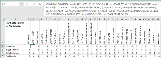
Even though it’s long, it’s not all that complicated:

1. At the top level, it’s a SUM of 5 things – the comparisons of the 5 attributes for the pair of cards.
2. Each comparison is an IF that returns 1 if the row’s card beats the column’s card for a given attribute, and 0 if it doesn’t.
3. To get the value of the Nth attribute for the row’s card, it does a VLOOKUP using the row label to find a row in the cards tab (where the data is in the region A2:F31), and then pick the N+1th column in that row (skipping the person’s name).
4. The value of the Nth attribute for the column’s card is very similar, just using the row heading.

Step 2 – calculating the net score for a pair

On the scores sheet I listed out all pairs.  To start with I created the numbers 1-30 in column 2, and then copy / pasted it to have 30 copies altogether.  I then deleted 1 from copy 1, 2 from copy 2 and so on.  I also pasted 1 in column 1 next to copy 1, 2 in column 1 next to copy 2 etc.  This was the most tedious part, where I wondered if I should be doing this via a program, but it didn’t take too long, particularly as I could use the feature where you could select some cells that had values (e.g. 1 then 2) and extend the selection over empty cells and Excel would fill in the empty cells by extrapolation, in my case 3, 4 etc.

I then used OFFSET and the values in those columns to bring in the names from the cards sheet.  I used OFFSET and the values in a similar way to bring in the pair’s scores from the pairs sheet.  I then subtracted one score from the other to create the net score.

Step 3 – calculating an average net score for a card

The rows in the score sheet are sorted by card A’s name and then by card B’s name.  This means I could use the SUBTOTAL feature to calculate the average for each card A.  At each change in the value in column C, it would calculate the average value in column G.  These values were given in new rows added by Excel at the end of a run of identical values in column C.  Excel also created a control (the |1|2|3| boxes on the left edge of the image above) to let you expand or contract the structure so that you could e.g. see just the averages rather than the details.

This gave me the values I wanted, apart from two problems:

1. The averages were intermingled with the details.  If I hid the details they were still there if I copy / pasted the averages to another sheet.
2. The averages’ labels were the person’s name followed by ” Average”.

To fix the first problem, I hid the details and then selected only visible cells.  I then copy / pasted the values into a new sheet.  I then did a find and replace, to replace ” Average” with “”, which deleted the stuff I didn’t want.

Step 4 – drawing the graph

The graph I picked was a line graph with markers.  I set the line to be No Line, and then increased the size of the markers.

That’s it!

The investigations re-used the sub-total technique, but instead of calculating an average per card, it calculated the number of rows with each number of gold medals.  (I just copy / pasted the golds column from the cards sheet into a new one, sorted it, and then did the sub-total.)  The graphs are 100% stacked column charts.