Recursion and iteration – an introduction to recursion

This is the second article in a series about recursion and iteration.

1. Introduction to iteration
2. Introduction to recursion
3. Mutual recursion and tail recursion
4. Blurring the lines
5. Loop unrolling

I will assume that you have already read the article on iteration, and this article will focus on recursion. Like iteration, recursion is a way of repeatedly doing the same or similar work, so that the sum of the repetitions solves a bigger problem. However, the way it works is different.

Counting descendants

Imagine you have a large family tree, and you want to count how many people are descended from someone on the tree. A way of counting this could be described as:

Number of descendants = Number of children they have + number of descendants each of their children has

This is an example of recursion. Note that number of descendants is on both sides of the equation. Recursion means that the solution to a problem includes one or more copies of the problem. The one or more copies are hopefully smaller than the original problem in some way, so that you’re gradually breaking the problem down into smaller and smaller bits until you get to bits that are small enough to solve. At that point you can start assembling the solutions to all the small bits into solutions to bigger and bigger bits, until you end up with a solution to the problem you started with.

You could do other things on a family tree that would also be recursive. For instance, if you wanted to find the maximum age (either current or at the time of their death) among someone’s descendants you could do it like this:

Maximum age among descendants =

1. Find max_children = maximum age among children
2. For each child C, find max_C = maximum age among C’s descendants
3. Find the maximum among max_children and all max_C

This is also recursive – step 2 is also calculating the maximum age of someone’s descendants, but based on smaller family trees (one layer shorter).

Non-tree example – Fibonacci numbers

The previous examples are a bit misleading on their own. They are both based on a family tree, which happens to be a particular kind of tree (a common data structure in computing). A tree is a recursive data structure, and so it follows that working with one should involve recursive code. By recursive data structure I mean that its definition involves copies of itself – just as a parent node is the head of a tree, each of the parent’s child nodes is also the head of a slightly smaller tree.

The classic non-tree example of recursion is calculating numbers in the Fibonacci series. To calculate the nth number in the series – X_n :

• X₀ = 0
• X₁ = 1
• X_n = X_n-1 + X_n-2

which results in the series 0, 1, 1, 2, 3, 5, 8, 13, 21, 34, 55, 89…

Doing it in code

The Fibonacci example is relatively simple, so I’ll use it as the problem to solve in code. It will be in C#, but I hope the general principles will be clear to non-C# speakers. The first stage should be no surprise:

int fibonacci(int n)
{
    if (n == 0) { return 0; }

    if (n == 1) { return 1; }
}

This will work for the first two numbers in the sequence. I started with these two because there’s no recursion involved. These two cases (0 and 1) are called the base cases of the recursion. If the code reaches either of these cases it won’t go any deeper, but will instead start gathering up bits of the solution towards having a solution to the full problem.

The remaining bit is called the recursive step, and this acts as the engine of the recursion. How do you solve a problem in terms of simpler versions of the problem? It’s actually not all that complicated, even if it might look odd.

int fibonacci(int n)
{
    if (n == 0) { return 0; }

    if (n == 1) { return 1; }

    return fibonacci(n-1) + fibonacci(n-2);
}

Recursive code involves a function (or method or whatever else you call it) calling itself, usually with different parameters that somehow specify a simpler or smaller instance of the problem. You might be wondering how it keeps track of things, and I will come to that shortly. First I want to run through an example to show its To Do list, to confirm that this will solve the problem as we expect. Just to save space and typing, I’ll abbreviate fibonacci(n) to f(n). I’ll also add in square brackets to show which bits go together. Also, I’ll expand each term immediately and in parallel with every other term on the same line – in real life they will be expanded (processed) one at a time, unless you re-wrote the code to calculate things in parallel.

1. f(4) = [f(3) + f(2)]
2. f(4) = [[f(2) + f(1)] + [f(1) + f(0)]]
3. f(4) = [[[f(1) + f(0)] + f(1)] + [f(1) + f(0)]]
4. f(4) = [[[1 + 0] + 1] + [1 + 0]]
5. f(4) = 3

So it looks like this will do the right thing, at least for this example.

In the article about iteration, I said that unfortunately you don’t have anything that will stop you from writing a while loop or for loop that will run forever. A similar thing is true for recursion. If I passed the value -4 to the method above, it will loop forever. -4 will lead to recursive calls with -5 and -6 etc, and so the code will never reach any of the base cases (0 or 1), and will instead go on forever. While I’ve been using terms like simpler and smaller in a hand-waving way, unfortunately they have no robust definition, and your recursive steps aren’t checked that they will always head in the direction of simpler or smaller.

Keeping track of things

The fibonacci example above is almost as simple as it could be, but still raises an interesting question: How can the computer keep track of what n is? In more complicated examples, there would be other things it would need to keep track of – local variables defined inside the method.

This is where knowing a little of the internals of things will help. As it runs, the computer uses memory as working storage. Part of this memory it organises in the form of a stack. The stack is divided up into boxes or frames – each time a new method call happens, a new frame is put on top of the stack (pushing down or hiding what was already there). It’s like each method call starts on a fresh page in a notebook – the stack frame is the notebook page. The temporary values for that method call – such as parameters passed in, local variables defined inside the method – are stored in the stack frame. When the method returns to the thing that called it the top stack frame is removed or popped, leaving what was the second frame as the new top frame.

Notice that I didn’t say anything about whether the calling method and the called method were the same as each other or different. That’s because it doesn’t matter. Each time the fibonacci method calls itself, a fresh stack frame is put on top of the stack and the fibonacci method starts from its first line again, in the context of this fresh stack frame.

I’ll go through the previous example – fibonacci(4) – to illustrate what’s happening. If you look at all the times that the method is called, you get a tree diagram like this:

The overall goal is to calculate f(4), and to accomplish this it calculates f(3) and f(2) etc. I’ve numbered each call to separate out the 2 instances of f(2), the 3 instances of f(1) and the 2 instances of f(0). If you look at the pattern of stack frames over time, it will look like this:

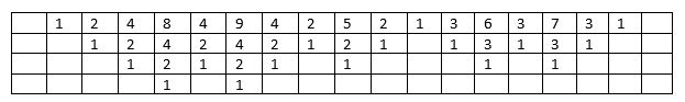
Time goes from left to right, and each column shows the stack at one point in time. The numbers refer to the stack frame for each node in the tree above. The top frame on the stack is the top row of the table – only this frame is accessible to the code.

The stack starts empty (it wouldn’t in reality, but I’m doing it to make things clearer). When f(4) is called, a new frame is put on the stack. Among other things, this will hold the fact that n=4 in this context. As I mentioned earlier, the two smaller calls – f(3) and f(2) happen one after the other rather than at the same time. So, f(3) is called and its stack frame is added to the stack (frame 2). In this stack frame, n=3. The process repeats two more times – the first part of calculating f(3) is to calculate f(2), so stack frame 4 is added, and to calculate f(2) we need to first calculate f(1) so stack frame 8 is added.

At this point we hit a base case of the recursion. We don’t need to make any further recursive calls as we know that f(1)=1. When this method call returns, its stack frame (frame 8) is popped off the stack, uncovering frame 4 and the results of f(1) can be added to frame 4. Frame 4’s work isn’t finished yet, and a call to f(0) is made, resulting in frame 9 being added and so frame 4 is pushed down again. f(0) is another base case so there’s no further recursive calls, frame 9 is removed when f(0) returns with the answer 0. Frame 4 now has all it needs to compute its result, which is 1+0=1.

Frame 4 was to compute f(2), which was in turn the first part of computing f(3) for frame 2. When f(2) returns with the answer 1, its frame is removed from the stack, leaving only frames 2 and 1. We now go deeper again to compute f(1), as that’s the second half of computing f(3). I won’t go through the details of the remaining steps, but I hope you can follow how the stream of activity and its accompanying changes to the stack will go.

Summary

Recursion is a way of tackling problems whose solution can be expressed in terms of a simpler or smaller version of the problem. In terms of code, it’s achieved by a method calling itself. For the recursion to keep going, you need a recursive step (the method calling itself). So that it doesn’t go on forever, you also need one or more base cases where certain inputs lead to no further recursion.