Fuzzy matching – example algorithms

This is the second article in a short series on fuzzy matching: 

• Introduction 
• Example algorithms 
• Testing and context 

In this article I will go into three algorithms that are examples of fuzzy matching – Levenshtein distance, Dynamic Time Warping (DTW) and Hidden Markov Models (HMMs). 

Levenshtein distance 

The Levenshtein distance is a way to do fuzzy matching between two text strings. It gives a score that’s zero or greater that shows the distance between the two strings.  I.e. zero means the strings are identical, and the score increases the more the strings are different from each other. 

The score increases by one for each one-character change you have to make so that one string is identical to the other. The one-character changes you can make are: 

• Delete a character from anywhere (shuffling the remaining bits together to make one string again) 
• Insert a character into anywhere (the existing characters move apart to make room) 
• Replace any character with a different character 

Therefore, the distance between bead and beak, bad and beard is one: 

• bead -> beak – replace the d with k 
• bead -> bad – delete e 
• bead -> beard – insert r 

The biggest score you could get is the length of the longer string, e.g. comparing abc and pqrst gives the distance 5: 

• Replace the a, b, c with p, q, r -> 3 changes 
• Add s, t -> a further 2 changes 

The main difficulty in computing the Levenshtein distance is that there are usually many options to convert one string to the other, and you need to find one of the options that gives the smallest distance.  For instance, in the abc/pqrst example you could delete all the characters abc and then add pqrst. This is valid, and gives a distance of 8 (3 deletions plus 5 insertions). However, there’s a different option for the same two strings as we saw that gives a lower score. 

This is a general pattern with fuzzy matching – they often involve searching for the best match among a series of candidate matches. This can make them more expensive to compute than conventional matching.  For instance, if you were to do a conventional match between bead and beard it would involve comparing corresponding characters from the two strings: 

1. b and b -> identical but there’s more to compare, so continue
2. e and e -> identical but there’s more to compare, so continue
3. a and a -> identical but there’s more to compare, so continue
4. d and r -> different, so stop and say that the strings are different

That’s it – there are no other candidate matches to do. 

A simple but inefficient way to compute the Levenshtein distance between two strings is as shown below (taken from Wikipedia). It’s recursive, so there are two terminating cases and a pair of propagating cases, one of which has three sub-cases. The algorithm compares both strings left to right, by repeatedly comparing the first character in each, then throwing it away and repeating the process on the remainder. 

Some notation: 

• |a| = number of characters in string a 
• a[0] = the zeroth i.e. first character in string a 
• tail(a) = the string a after its zeroth character has been removed
• lev(a,b) = the Levenshtein distance between strings a and b

With that notation established, here’s a pseudo-code, i.e. hand-wavy, description of the algorithm:

lev(a,b) 
    if |a| == 0 return |b|
    if |b| == 0 return |a| 

    if a[0] == b[0] return lev(tail(a), tail(b)) 

    distanceWhenDeletingFromA = lev(tail(a), b) 
    distanceWhenInsertingIntoA = lev(a, tail(b)) 
    distanceWhenSubstituting = lev(tail(a), tail(b)) 

    return 1 + min(distanceWhenDeletingFromA, 
                   distanceWhenInsertingIntoA, 
                   distanceWhenSubtituting)

There is a more efficient approach based on iteration, that is similar to the dynamic time warping technique described in the next section. 

In some situations you might want to normalise the Levenshtein distance, e.g. by dividing it by the length of the longer string.  This will give a score in the range 0 to 1. The reason why you might want to do this is if you’re interested in computing what fraction of the strings being compared is different, rather than the absolute size of the difference.  E.g. abc/xyz and advantage/advantageous both have a raw Levenshtein distance of 3, but a normalised distance of 1 and 0.25 respectively. 

Dynamic time warping 

Dynamic time warping (DTW) is a way of computing the best match between two series of data, where the two series don’t necessarily have the same length. (It isn’t, to my knowledge, anything to do with the Rocky Horror Picture Show.) 

The name is linked to the fact that the series of data might be showing how something changes over time, e.g. stock prices or the volume of audio recordings. However, the series don’t have to be spread out due to time; they could show how something varies in space or some other dimension. 

If the series are different lengths, one approach would be to just chop off part of the beginning and/or end of the longer series until the two series are the same length and then do a simple comparison on what’s left. Once one series has been trimmed, the simple comparison would take the first value from one series and compare it to the first value from the other series, then the second value from one series with the second value from the other series etc. The overall comparison for the series could be the sum (or possibly average, max or some other function) of the distances from each comparison of a pair of values.  

However, with DTW you can effectively stretch and squash time, so that all of both series can be used in the comparison. The first value from one series is compared to the first value of the other series, and the pair of last values from the series are compared to each other. For the values in between, time is treated as in Dr Who (wibbly wobbly timey wimey stuff) – any value from one series can be compared to any value from the other. 

Note that the only thing changed is how values are paired up – the way you compare a given pair of values is unchanged by DTW cf. any simpler way of comparing the series. Also, note that time can be warped but it can’t be cut – you can’t skip values in either series. All values need to be compared to at least one value in the other series. 

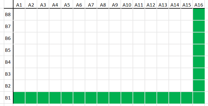
The diagrams below show different ways that two series of different lengths might be compared. The two series A and B represent the two axes of the chart. A1, A2 etc. are the values in A and B1, B2 etc. are the values in B. Each cell in the chart represents the comparison of one value from each series.  The highlighted cells represent the best match. 

One of the series is twice the length of the other, so you might expect each value from the shorter series to be compared to two values from the longer series.  This would be sensible if one represents someone speaking at half the speed that they did in the other data series. 

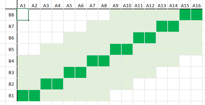
However, if they didn’t do a simple slowing down, but slowed down in some places and sped up in other places, the best comparison might be more complicated, as shown in this diagram.

The most extreme is when all the values from series A are paired up with the first value of series B, and then the last value of A is paired up with all the values from series B i.e. the path of this match goes around the edge of the rectangle or matrix of comparisons.

The charts above represent how DTW is calculated. If the series have lengths M and N, then there is an array of size M+1 x N+1. The value in cell (x,y) holds the total difference of the best alignment of series A up to its x^th value with series B up to its y^th value. So cell (M,N) is the comparison for the two series overall. 

The simplest approach is to work through all possibilities, starting in the bottom left and aiming for the top right. In general, the comparison up to and including the pair (x,y) is the sum of: 

• the difference between A[x] and B[y] 
• the comparison following the best path up to (x,y) 

There are three options for the last part, based on whether we are moving on from a previous pair to (x,y) by advancing through series A, series B, or both series. Or, in terms of the diagrams above, whether we are moving to a given cell by moving up, right, or diagonally up and right. 

If A and B are small, it might be quick enough to simply compute all the chart, i.e. all possible pairings. However, as A and B get big, the number of pairings grows quickly. One approach to taming this is to set a limit on how far we are prepared to deviate from the diagonal line of the first diagram above towards the extreme case of the last diagram. 

Effectively we draw a thicker diagonal line (the pale green region in the chart below) around the one from the first diagram, which defines a set of values that we’re prepared to calculate and leave all other values uncalculated. The path of the best match can wiggle around the inner diagonal line a little, but not so much that it leaves the region of the thicker diagonal line. 

There are more details that I’m skipping over, but are covered in articles that specialise in just DTW. 

HMM

A Hidden Markov Model or HMM is one way of generalising a finite state machine (FSM). (If you’re new to finite state machines, please look at my article on FSMs.) 

In an FSM there are states, and the system is in one state at a time. When an input is received, this might cause the system to move to a new state. (This is possible only if there is a transition or arrow between the two states, where this transition is labelled with the relevant input.) If at the end of the series of inputs the state that the system is in is a member of the set of accepting states, the series of inputs is valid. If the inputs run out before the system is in an accepting state, the series of inputs is invalid. 

An HMM is like an FSM in that: 

• There are states and the system is in one state at a time; 
• There are transitions between states; 
• There is a set of messages (like the inputs of an FSM), sometimes called observations. 

However, there are also two sets of probabilities: 

1. Each transition is labelled with a probability, that says how likely it is for the system to move along the transition to the new state;
2. There is a probability linking each state with each possible input that says how likely that input is given the system is in that state.

This pair of probabilities allows for two dimensions of fuzziness: 

1. The sequence of states that the system goes through
2. The series of messages that the system can handle while it passes through those states

The idea is that there’s a set of observations that you can see, that are linked to a state machine that you can’t (the HMM). The creation of the probabilities is non-trivial, and this is usually done by training the model on some training data. This is the most mathematically advanced of the three fuzzy matching algorithms in this article – for more details I suggest you look at articles elsewhere on HMMs.