Balanced trees

In a previous article on complexity, i.e. performance trends in code, I said that trees can be useful ways of storing data, but they only work if they’re reasonably well balanced. In this context, balanced means that no path from the root node of the tree to a leaf node is much longer than any other path.  Balanced trees tend to be symmetrical and bushy, rather than long and straggly.

Balanced trees are great, but how do you encourage a tree to be balanced?  In this article I will describe one approach to this, which is the 2-3-4 tree, which is a special case of the B-tree.  I’ll explain 2-3-4 trees in general and then give examples of building two trees.  Comparing the two trees will touch on another common issue in computing, which is allocating storage in blocks and how efficiently those blocks are used.

Recap of binary trees

Before we get into 2-3-4 trees, here’s a recap of binary trees.  Binary trees are simpler than 2-3-4 trees, which makes them easier to understand but also prone to becoming unbalanced.

A binary tree is made up of nodes connected to up to two other nodes (hence their name).  Each node holds a value – for the sake of this article I will assume all values in trees are integers, but they could be anything that could be put into an order – strings, floating point numbers, complex data types if values of that type can be described as greater or less than other values, etc.

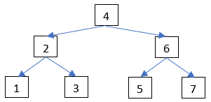
The tree is usually drawn upside down – the single root node is at the top, and the two nodes it’s connected to (its children) are below it, and the nodes with no children at the bottom are called leaf nodes.  The only other important thing is that the value in the left child of a node is less than the node’s value, and the value in the right child is greater than the node’s value.

The rule about left and right children means that searching for a value in a binary tree can be much quicker than if the same values were in a list.  The way to search is:

1. Start at the root node.
2. If the current node is null or empty, return with the news that the value is missing.
3. If the current node is the value you’re looking for, return it and stop.
4. If the value you’re looking for is less than the current node’s, repeat from step 2 using the left child as the current node.
5. If the value you’re looking for is greater than the current node’s, repeat from step 2 using the right child as the current node.

Step 2 might seem a bit odd, but it handles both the cases that a node has no left child or no right child.

The reason why a balanced binary tree is good for storing data (actually, for storing it in a way that means looking for things later is efficient) is that each time around the loop above, you discard half the remaining options.  If the value you’re looking for is less than the current node’s value, you don’t look at the right child or its descendants (and vice versa for the left child).

When you add a new value to a binary tree, you look for the value in the tree and add the new value to the node where you give up.  I.e. you add the new value to the node that’s the nearest miss for the new value (as far as the tree’s concerned, rather than e.g. the positions of the nodes’ values on the number line).

So, as described in the article on complexity, the pathological case for binary trees is adding numbers in the order 1, 2, 3, etc. (Starting with the maximum value and adding in descending order is an equivalent pathological case.) Each new node becomes the new right child of the right-most leaf node, so the tree turns into a list, with the worse performance for searching that comes with a list.

More complex nodes

Before we get to the full 2-3-4 tree stuff, a useful chunk of information to help explain that is what happens when a node can hold more than 1 value.  There’s no limit to the number of values a node can hold, but a 2-3-4 tree can hold 1-3 values per node.  As you will see, there’s a relationship between the number of values in a node and the maximum number of children it can have – a node with N values can have up to N+1 children.  Therefore, the 1-3 values in a node for a 2-3-4 tree means a node can have 2-4 children (hence its name).

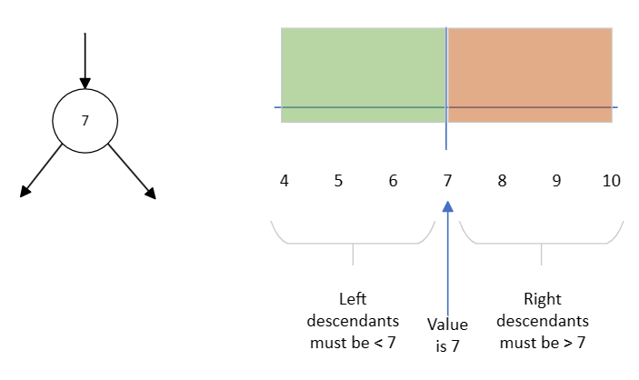
If you look at a number line, the single value in the node of a binary tree divides the line into 2 areas.  The left child and all its descendants must be in the part of the number line to the left (less than) the node’s value.  Similarly, the right child and all its descendants must be in the part to the right.

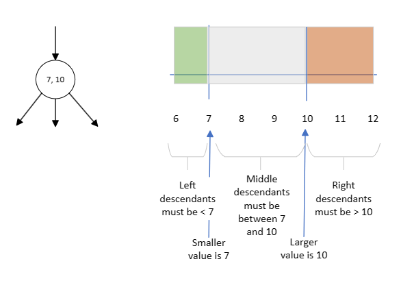
If you have 2 values in the node, this divides the number line into 3 areas.  These are the areas for the left child and its descendants, the middle child and its descendants and the right child and its descendants.  The areas are:

1. Less than the smaller node value
2. Between the node values
3. Greater than the bigger node value

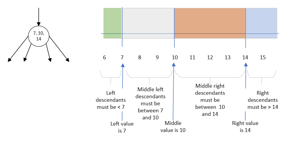
You might have spotted the pattern already, but this is what happens if you have 3 values in a node.  The values divide the number line into 4 regions:

1. Less than the smallest node value
2. Between the smallest and middle node values
3. Between the middle and biggest node values
4. Bigger than the biggest node value

Building 2-3-4 trees

A 2-3-4 tree is a tree with nodes that hold 1-3 values and hence have 2-4 children.  Generalising from binary trees to 2-3-4 trees on its own isn’t enough to keep trees balanced.  As well as a difference in the nodes, it’s important to also have a difference in the rules for building trees.  (There are also differences in the rules for deleting and updating values, but I’ll leave them out as this article is already quite long.)

If you’re trying to add a new value to an existing tree:

1. Start with the root node.
2. If the current node has children, find the appropriate+ child and repeat from step 2.
3. If the current node has 3 values, split them into 3 separate parts.  The middle value is added to the parent node.  If there is no parent (because the current node is the root node), create a new root node for the middle value.  The remaining values in the current node become 2 separate children of the parent node. Move up to the parent node and if it now has 3 values, repeat this step.
4. Now splitting has finished, start going back down the tree at step 2.
5. When you finally get to a node that has no children and 1 or 2 values, add the new value.

+ appropriate is shorthand.  The node can have 1-3 values, and so will have 2-4 children.  The child to pick depends on the number of values in the node and how those values compare to the value you’re trying to add, as described in the previous section.

This might be a bit hard to follow, so here’s a summary and I will go through some examples below:

1. New values are added to leaf nodes and not internal nodes;
2. If the leaf node you want to add to is full, it’s split into 2 and its middle value is pushed up to its parent.  Internal nodes can’t be left with 3 values, so keep splitting and pushing the middle value upwards until you get to an internal node with only 1 or 2 values.

For me, it’s step 2 that’s the biggest difference from binary trees.  Existing values are moved within the tree, as well as new values being to leaf nodes.

Example tree: adding numbers 1-31 in ascending order

This is the pathological case from the previous article on complexity.  Snapshots of the process are presented below, and you can visit an animation where you can step through the whole process.

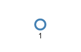
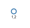
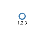
The numbers 1-3 are quite straightforward – a new node is created to hold 1, and this also receives 2 and 3:

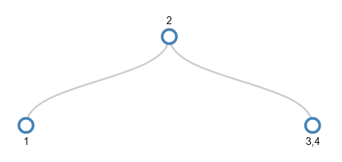
When we want to add 4 there’s no room in the node.  So, the middle value (2) is pushed up a level, but as there’s no parent node, a new parent node is created.  The remaining values (1 and 3) become separate children of the parent.

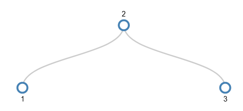
This leaves a node with space to add 4 – the node that now holds only 3.

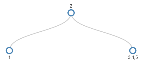
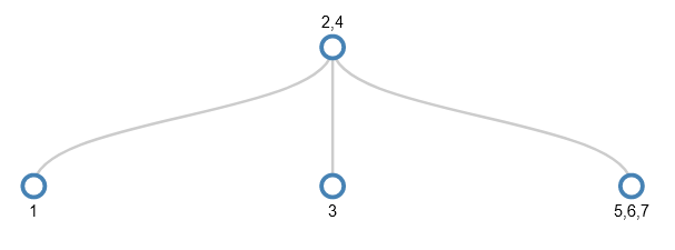
5 is added by simply adding it to 3 and 4, but when we come to add 6 there’s a full node again where we want to add the new value (the 3,4,5 node).

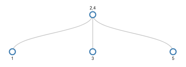
So, again the middle value (4) is pushed up a level (which exists this time).  This turns the parent node into 2,4 and turns the remaining bits of the 3,4,5 node into 2 separate children of this parent.  The other child (the 1 node) stays as it is, so the tree after splitting looks like this:

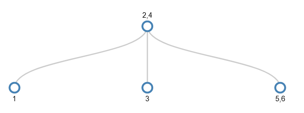
6 can be added to the 5 node now it has space.

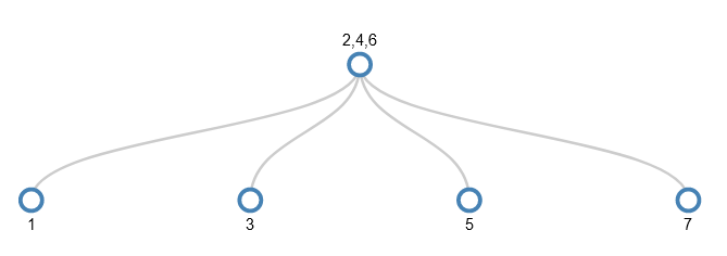
You might see a pattern here.  Because values are being added in ascending order, they will always want to be added to the bottom right node.  When this becomes full, we make space by pushing the middle value up a level and making new smaller nodes.  This continues until we want to add 8.  The node we want to add to (5,6,7) is full, and its parent has 2 values.

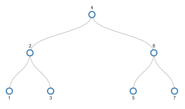
To make space in the target node, its middle value (6) is pushed up a level.  However, this leaves the parent as an internal node with 3 values (2,4,6) which isn’t allowed – only leaf nodes can have 3 values.  So the splitting continues – the middle value (4) is pushed upwards and the remaining values become its children.

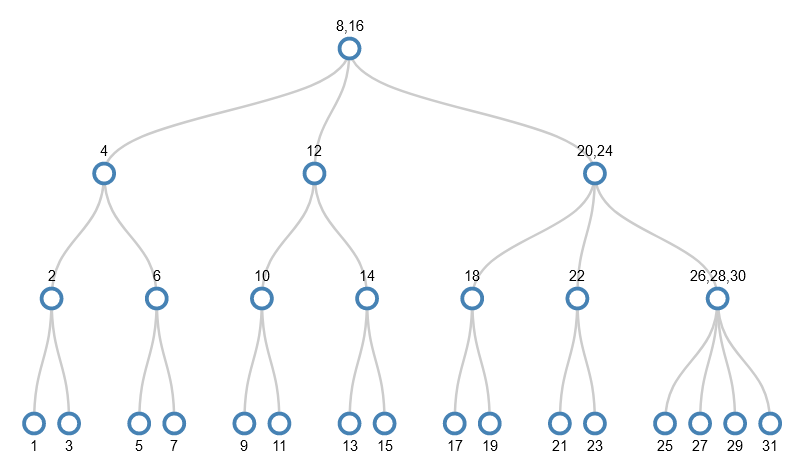
I’ll skip forwards to the point where the values 1-31 have been added and we want to add 32.  I won’t actually add 32, but show the splitting that happens to make the tree ready to accept 32.  It’s the equivalent of adding 1 to a number such as 9999.  Just as each digit in 9999 already holds as big a thing as it can (the value 9), each node in the path from the root node to the target leaf node is as full as it can be.  So the act of dealing with the smallest part (the rightmost digit in 9999 or the leaf node in the tree) has a ripple effect from one end to the other.

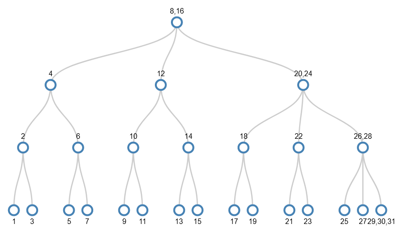
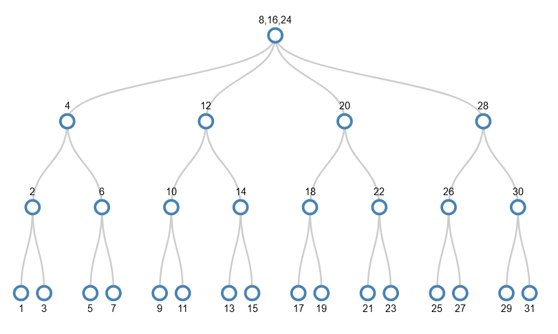
Despite the values being added in order 1-31, and hence always adding them to the bottom right node, the tree we get has some very interesting properties:

1. The bottom row (leaf nodes) has odd numbers, i.e. the gaps between numbers is 2;
2. In the next row up, the gap between numbers is 4;
3. In the next row up, the gap is 8;
4. In the next row up, the gap is 16;
5. The left-most value in each row is a power of 2.

Note that these are specific to this tree because of the order in which values were added.  The other example below doesn’t have these properties.  The same numbers are added, but in a different order.

Example tree: adding numbers 1-31 is random order

The same numbers are added, but in this order:

1, 27, 5, 23, 10, 9, 29, 26, 12, 8, 7, 3, 19, 20, 2, 21, 24, 22, 15, 6, 28, 13, 31, 17, 16, 30, 11, 18, 14, 4

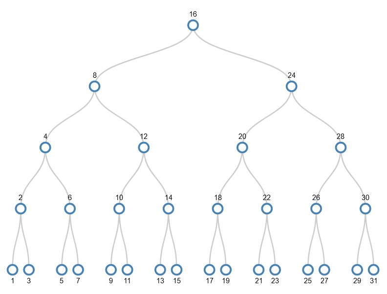
I won’t go through the stages here because the important parts are the same as before, but you can visit another animation of values being added to the tree in this random order.  The tree ends up looking like this

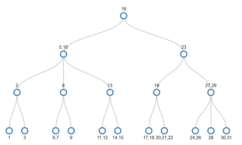
There are some interesting similarities and differences compared to the previous example:

• While the nodes in each level are in order smallest to biggest left to right, there’s no strict pattern to which values are in which level or the gaps between values in a given level;
• There are nodes with 2 or 3 values in them, whereas the previous tree had just nodes with 1 value in (it was a binary tree).  The average number of values per node in this tree is 1.6, and so there are fewer of them (19 rather than 31).

Allocating space in blocks

The difference between the two trees illustrates a more general point in computing – allocating space in blocks of fixed size.  In the case of the trees, the blocks are the nodes, which can hold 1-3 values.  In the first tree, each node holds only 1 value even though they can store 3.  In the second tree, the nodes hold 1-3 values and so fewer nodes are needed to store the same number of values.

In the case of files on a disk, or indexes and tables in a database, the blocks are chunks of storage that could be e.g. 8k big.

The basic problem in both is that there is something (a tree, a file, a database table) that needs space, but we don’t know how much space.  The thing might shrink or grow, or its contents change over time.  Finally, there are likely to be several things (trees, files, tables) we need to store at the same time.  So we need to balance flexibility with efficiency.

The smaller each block is, the more blocks we need to store a given amount of stuff.  Each block has a cost in terms of overhead – this could be pointers to child nodes in the case of a tree, or a look-up table in the case of files in a file system.  However, the smaller each block is, the smaller the worst case is for how much space is wasted.  The maximum that could be wasted is 1 less than the size of the block – where 1 means 1 byte in the case of a block of file system and 1 value in the case of a tree node.  However, this assumes that occasionally data is shuffled between blocks, to turn e.g. 6 half-filled blocks into 3 fully-filled blocks.

This shuffling of things to reduce wasted space is known as defragmentation.